
July 13, 2026
Scott Routledge
In this post, we demonstrate the first fully open source text-to-analytics stack for Apache Iceberg data in a simple workflow.
This stack brings together three open source technologies: PyDough, the trusted answer layer that translates natural language into validated analytical logic; BodoSQL, the distributed query engine that executes those queries with low latency; and Apache Iceberg, an open table format for managing large datasets. Together, they provide the foundation for natural language analytics that is not only easy to use, but also verifiable, performant, and scalable.
The architecture is designed to solve the two core challenges of production text-to-analytics: trustworthiness and scalability. LLMs make it easy to ask questions of data by translating natural language into queries that can be executed on a database, but they provide no guarantee that generated queries faithfully capture a user's intent. And because analytics is inherently iterative, every query must execute quickly enough to support interactive exploration. By pairing a trusted semantic layer with a high-performance analytics engine, the stack addresses both challenges.
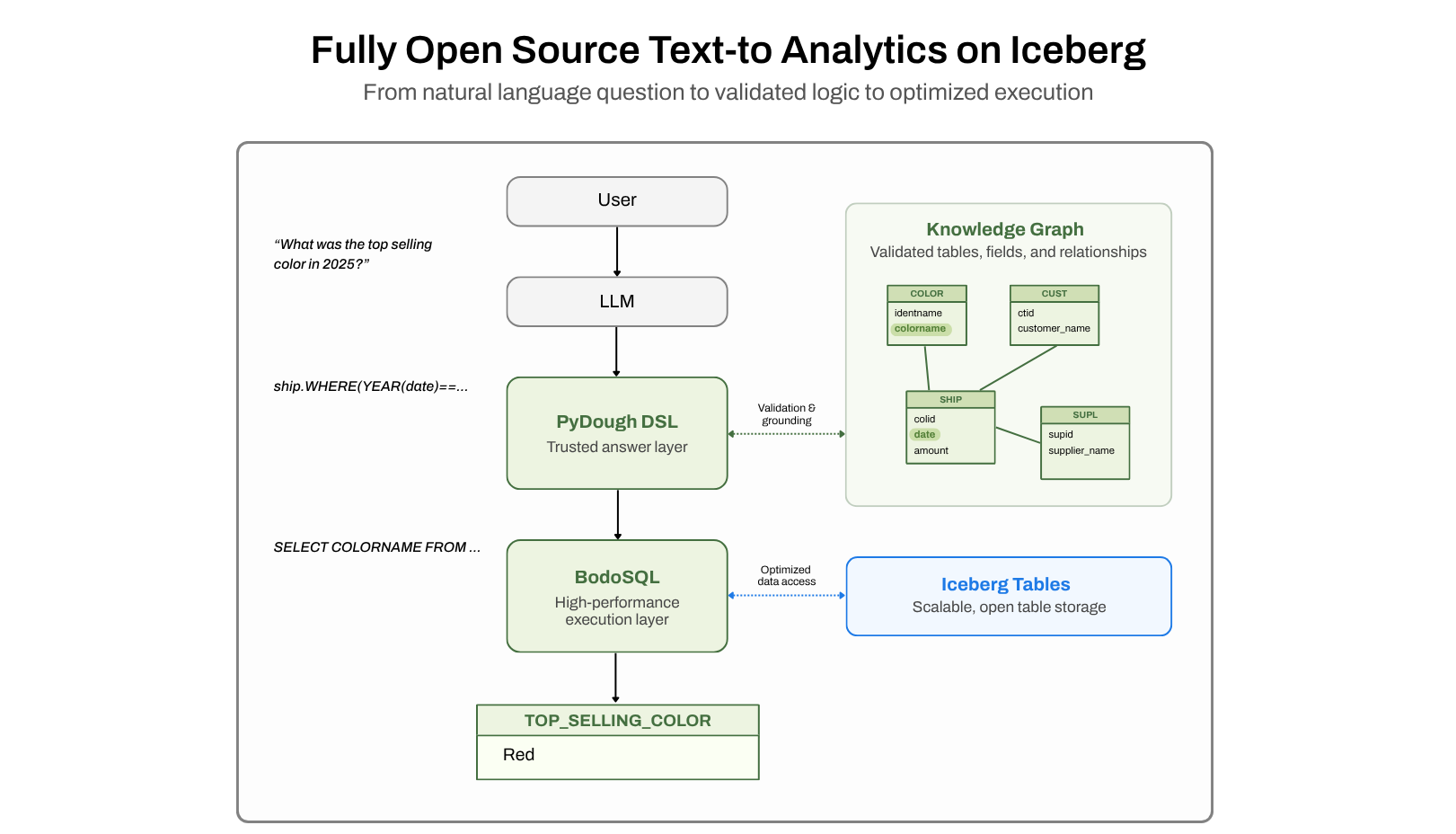
We'll build the complete workflow from scratch. Starting with a set of Iceberg tables, we'll connect them to BodoSQL, generate the PyDough knowledge graph that captures the database structure and relationships, and use an LLM to answer questions about the data using PyDough. Finally, we'll take a closer look at the BodoSQL execution engine to see how query optimization techniques such as filter pushdown, join reordering, and runtime join filters enable efficient execution over Iceberg tables.
By the end of this post, you'll have an end-to-end workflow that spans every layer of a modern analytics system—from data storage and distributed query execution to semantic validation and natural language interfaces—using entirely open source technologies.
You can install the required packages for this workflow, including PyDough, BodoSQL, PyIceberg and PyDough-analytics, with a single pip install line:
pip install "pydough-analytics[bodosql,iceberg,notebooks]"You will also need to install any packages for your LLM provider. By default, PyDough-analytics uses Google’s Gemini Enterprise Agent Platform (formerly Vertex AI), however, you can use a different model provider as long as it is compatible with aisuite. The workflow in this example uses gpt-5.5.
We begin the example by setting up an Iceberg database on our local filesystem using Bodo DataFrames to write Iceberg tables.
The database for this example comes from a synthetic “Colorshop” dataset, which includes 4 tables:
COLOR table contains: A color identifier, color name, hex value, R,G,B valuesCUST table contains: Customer name, Customer IDSUPL table contains: Supplier name, Supplier IDSHIP table contains: Shipment ID, color identifier, customer ID, supplier/company ID, purchase date, amount of paint purchased, priceThe full script to generate the dataset can be found in Appendix A. below or in the notebook for this workflow.
Next, we rewrite the Colorshop dataset, stored as Pandas DataFrames, into Iceberg tables stored on the local filesystem using Bodo’s Directory Catalog. For the “Shipments” table, we also show how you can add partition fields for Company ID and Color ID.
import os
import bodo.pandas as bd
from pyiceberg.partitioning import PartitionField, PartitionSpec
from pyiceberg.transforms import IdentityTransform, BucketTransform


iceberg_warehouse = "iceberg_warehouse"


table_names = ["COLOR", "CUST", "SUPL", "SHIP"]
tables = [color_df, customers_df, suppliers_df, shipments_df]


if not os.path.exists(iceberg_warehouse):
   bd.from_pandas(color_df).to_iceberg("COLOR", location=iceberg_warehouse)
   bd.from_pandas(customers_df).to_iceberg("CUST", location=iceberg_warehouse)
   bd.from_pandas(suppliers_df).to_iceberg("SUPL", location=iceberg_warehouse)


   # Partition shipments table by company, color
   spec = PartitionSpec(
       PartitionField(4, 1001, IdentityTransform(), "com_part"),
       PartitionField(2, 1002, BucketTransform(10), "col_part")
   )
   bd.from_pandas(shipments_df).to_iceberg(
"SHIP", location=iceberg_warehouse, partition_spec=spec
   )
After we create our Iceberg database, we need to connect to it with BodoSQL. Here, we use BodoSQL’s FilesystemCatalog to query the Iceberg tables written in the previous step:
from bodosql import BodoSQLContext, FileSystemCatalog


catalog = FileSystemCatalog(os.path.abspath(iceberg_warehouse))
bc = BodoSQLContext(catalog=catalog)
To make sure our context is constructed correctly, we can execute a simple query using the BodoSQLContext.sql() function:
bc.sql("SELECT * FROM SHIP LIMIT 5")Output:
| | SID | COLID | CUSID | COMID | DOS | VOL | PRC |
|---:|------:|:-------------|--------:|--------:|:-----------|------:|------:|
| 0 | 19 | jade | 13 | 1 | 2024-01-01 | 2 | 28.6 |
| 1 | 30 | jade | 11 | 1 | 2024-01-01 | 2 | 28.6 |
| 2 | 105 | red_pigment | 8 | 1 | 2024-01-01 | 2 | 25.6 |
| 3 | 154 | blond | 15 | 1 | 2024-01-01 | 0.5 | 6.9 |
| 4 | 181 | carmine_pink | 7 | 1 | 2024-01-01 | 1 | 20.47 |To connect to your own database using BodoSQL, refer to this documentation page on creating a catalog for different types of databases. In addition to Iceberg tables, BodoSQL also supports querying Pandas DataFrames, raw CSV or Parquet files, and data stored in Snowflake and AWS Glue Catalogs.
Before we can use an LLM and PyDough on our database, we need to create two metadata files:
from pydough_analytics.commands.generate_md_cmd import generate_markdown_from_config


db_name = "COLORSHOP"
generated_kg_path = "generated_color_graph.json"
generated_md_path = "generated_color.md"
generate_markdown_from_config(db_name, json_path=kg_path, md_path=md_path)
Now that we have created the PyDough metadata and BodoSQLContext, we are finally ready to ask an LLM a question about this dataset. The following code creates an LLMClient and calls our model:
from pydough_analytics.llm.llm_client import LLMClient


provider="openai"
model="gpt-5.5"


client = LLMClient(
   provider=provider,
   model=model
)


question = "Find the 3 paint colors Quentin Sharma purchased the most of and how much volume was purchased for each."


result = client.ask(
   question=question,
   kg_path=kg_path,
   md_path=md_path,
   db_name=db_name,
   bodosql_context=bc,
)
The ask() function will return a Result object, which contains the generated PyDough code along with the LLM’s explanation of what it does, and the answer DataFrame. If there was an exception raised during execution, the results will include the exception message:
if result.df is None:
   print(result.exception)
else:
   print(result.code)
   print(result.full_explanation)
   print(result.df)
Output:
quentin_sharma_shipments = ship.WHERE(
(customer.cstfname == "Quentin") & (customer.cstlname == "Sharma")
).CALCULATE(
paint_color=color.colorname
)
result = quentin_sharma_shipments.PARTITION(
name="color_groups",
by=paint_color
).CALCULATE(
paint_color=paint_color,
total_volume_purchased=SUM(ship.vol)
).TOP_K(
3,
by=total_volume_purchased.DESC()
)
This code:
1. Starts from the `ship` collection because purchases are represented as shipments.
2. Filters shipments to only those purchased by customer **Quentin Sharma**.
3. Extracts the paint color name from the related `color` record.
4. Groups shipments by paint color.
5. Sums the purchased volume for each color.
6. Returns the top 3 colors by total purchased volume.
| PAINT_COLOR_NAME | PURCHASED_VOLUME |
|------------------|-----------------:|
| Flamingo Pink | 66.5 |
| Beau Blue | 65.0 |
| Dark Powder Blue | 62.5 |Under the hood, the ask() function extracts PyDough code generated by the LLM and uses PyDough to compile it to SQL. At this point, mistakes in the generated PyDough code, such as references to entities or relationships that do not exist in the knowledge graph, are caught before any execution happens. Once the code is compiled to SQL, it is executed using the provided BodoSQLContext, which returns a DataFrame. Here, we print the SQL generated in the previous example:
print(result.sql)
Output:

WITH _s2 AS (
  SELECT
    ship.colid,
    SUM(ship.vol) AS sum_vol
  FROM ship AS ship
  JOIN cust AS cust
    ON cust.cstfname = 'Quentin' AND cust.cstid = ship.cusid AND cust.cstlname = 'Sharma'
  GROUP BY
    1
)
SELECT
  color.colorname AS paint_color_name,
  COALESCE(_s2.sum_vol, 0) AS purchased_volume
FROM _s2 AS _s2
JOIN color AS color
  ON _s2.colid = color.identname
ORDER BY
  2 DESC NULLS LAST
LIMIT 3
Now that we understand how LLMClient.ask() works, let’s take a look at another example demonstrating how the BodoSQL backend executes PyDough-generated SQL efficiently over Iceberg tables by highlighting some key optimization the BodoSQL planner can perform. In this example, we ask:
Which light-colored paint shipments generated the highest revenue for Pallette Emporium and Rainbow Inc.? For each shipment, provide the customer, price, color and company name.
Here, "light-colored paint shipments" means shipments where red, blue and green values are all greater than or equal to 100.
We use a hand-crafted Pydough query to avoid randomness from the LLM and keep the example cleaner. To run the following Pydough code in a notebook, you will first have to load the Jupyter extension, load the metadata graph and connect to our BodoSQL context from the previous step:
import pydough
%load_ext pydough.jupyter_extensions


pydough.active_session.connect_database("bodosql", context=bc)
pydough.active_session.load_metadata_graph(kg_path, db_name)
We construct the following query by first filtering shipments based on the company name as well as the color to find only light colored shipments from Pallette Emporium and Rainbow Inc. Then, we use the filtered shipments result to find the customer name, price, color and company name for each shipment and sort by price.
%%pydough


selected_shipments = ship.WHERE(
   ISIN(suppliers.supname, ["Pallette Emporium", "Rainbow Inc."]) &
   (colors.b >= 100) & (colors.g >= 100) & (colors.r >= 100)
)


result = selected_shipments.CALCULATE(
   shipment_id=sid,
   customer_name=JOIN_STRINGS(' ', customers.cstfname, customers.cstlname),
   color_name=colors.colorname,
   company_name=suppliers.supname,
   price=prc,
).TOP_K(
   5,
   by=price.DESC(),
)
Similar to the LLM example, we can view SQL that’s generated from this query using our knowledge graph:
print(pydough.to_sql(result))Output:
SELECT
ship.sid AS shipment_id,
CONCAT_WS(' ', cust.cstfname, cust.cstlname) AS customer_name,
color.colorname AS color_name,
supl.supname AS company_name,
ship.prc AS price
FROM ship AS ship
JOIN supl AS supl
ON ship.comid = supl.supid AND supl.supname IN ('Pallette Emporium', 'Rainbow Inc.')
JOIN color AS color
ON color.b >= 100
AND color.g >= 100
AND color.identname = ship.colid
AND color.r >= 100
JOIN cust AS cust
ON cust.cstid = ship.cusid
ORDER BY
5 DESC NULLS LAST
LIMIT 5
We can also look at the optimized logical plan that BodoSQL will execute based on the generated SQL:
print(bc.generate_plan(pydough.to_sql(result)))
CombineStreamsExchange
  BodoPhysicalProject(SHIPMENT_ID=[$0], CUSTOMER_NAME=[CONCAT_WS(' ', $4, $5)], COLOR_NAME=[$3], COMPANY_NAME=[$2], PRICE=[$1])
    BodoPhysicalSort(sort0=[$1], dir0=[DESC-nulls-last], fetch=[5])
      BodoPhysicalProject(SID=[$0], PRC=[$2], SUPNAME=[$3], COLORNAME=[$4], CSTFNAME=[$6], CSTLNAME=[$7])
        BodoPhysicalJoin(condition=[=($5, $1)], joinType=[inner], JoinID=[0])
          BodoPhysicalProject(SID=[$0], CUSID=[$2], PRC=[$3], SUPNAME=[$4], COLORNAME=[$6])
            BodoPhysicalJoin(condition=[=($5, $1)], joinType=[inner], JoinID=[1])
              BodoPhysicalProject(SID=[$0], COLID=[$1], CUSID=[$2], PRC=[$4], SUPNAME=[$6])
                BodoPhysicalJoin(condition=[=($3, $5)], joinType=[inner], JoinID=[2])
                  IcebergToBodoPhysicalConverter
                    IcebergRuntimeJoinFilter(joinIDs=[[0, 1, 2]], ...)
                      IcebergFilter(condition=[AND(IS NOT NULL($1), IS NOT NULL($2), IS NOT NULL($3))])
                        IcebergTableScan(table=[[., ., SHIP]], Columns=[[SID, COLID, CUSID, COMID, PRC]], Iceberg=[true])
                  IcebergToBodoPhysicalConverter
                    IcebergFilter(condition=[AND(IS NOT NULL($0), SEARCH($1, Sarg['Pallette Emporium':VARCHAR(16777216)...])
                      IcebergTableScan(table=[[., ., SUPL]], Columns=[[SUPID, SUPNAME]], Iceberg=[true])
              IcebergToBodoPhysicalConverter
                IcebergProject(IDENTNAME=[$0], COLORNAME=[$1])
                  IcebergFilter(condition=[AND(>=($2, 100), >=($3, 100), >=($4, 100), IS NOT NULL($0))])
                    IcebergTableScan(table=[[., ., COLOR]], Columns=[[IDENTNAME, COLORNAME, R, G, B]], Iceberg=[true])
          IcebergToBodoPhysicalConverter
            IcebergFilter(condition=[IS NOT NULL($0)])
              IcebergTableScan(table=[[., ., CUST]], Columns=[[CSTID, CSTFNAME, CSTLNAME]], Iceberg=[true])
The logical plan for this query highlights several optimizations performed by the BodoSQL planner to minimize the amount of data that must be processed. The first is filter pushdown. Filters on both the Colors and Suppliers tables are pushed directly into the Iceberg scan, allowing irrelevant rows to be eliminated before they are read. For example, the filter on the Colors table produces:
IcebergFilter(condition=[AND(>=($2, 100), >=($3, 100), >=($4, 100), IS NOT NULL($0))])
For large datasets, filter pushdown can significantly improve performance by reducing the number of files that need to be scanned.
In addition to pushing filters into the scans, the planner determines an efficient join order using a cost-based dynamic programming algorithm. Rather than simply joining tables in the order they appear in the SQL query, BodoSQL chooses the order that minimizes the size of intermediate results. In this example, the large Shipments table is first joined with the small Suppliers table, which acts as a filter. The resulting dataset is then joined with the Colors table to further reduce its size before finally joining with Customers.
Because the planner joins Suppliers and Shipments first, it can apply an additional optimization: runtime join filters. Runtime join filters are generated from the values observed on the build side of a join and applied to the probe side while the query is executing. In this example, the filtered Suppliers table contains only two supplier IDs, allowing BodoSQL to discard Shipments rows that cannot possibly match. This runtime join filter can also be pushed into the Iceberg scan, and since Shipments is stored as an Iceberg table partitioned by supplier ID, approximately 60% of the table's files to be pruned before they are read.
In this post, we've shown how an LLM, PyDough, BodoSQL, and Apache Iceberg can work together to answer questions over large datasets stored in Iceberg tables. Each layer of the stack plays a complementary role in making the system both reliable and scalable:
Together, these components form an end-to-end architecture that combines the flexibility of natural language interfaces with the performance and trustworthiness required for production-scale analytics.
To try the workflow yourself, explore the open source projects behind the stack:
The colors CSV can be found here:
import datetime
import numpy as np
import numpy.typing as npt
import pandas as pd


datapath = "../data/datasets/colors.csv"


def generate_color_tables():
   color_df: pd.DataFrame = pd.read_csv(
       datapath,
       names=["IDENTNAME", "COLORNAME", "CHEX", "R", "G", "B"],
   )
   customers_df: pd.DataFrame = pd.DataFrame(
       {
           "CSTID": range(1, 21),
           "CSTFNAME": [
               "Alice",
               "Bob",
               "Charlie",
               "David",
               "Eve",
               "Frank",
               "Grace",
               "Heidi",
               "Ivan",
               "Janet",
               "Karl",
               "Leo",
               "Marcel",
               "Nina",
               "Oscar",
               "Peggy",
               "Quentin",
               "Rahul",
               "Sybil",
               "Trent",
           ],
           "CSTLNAME": [
               "Smith",
               "Johnson",
               "Williams",
               "Jones",
               "Brown",
               "Davis",
               "Miller",
               "Wilson",
               "Moore",
               "Taylor",
               "Anderson",
               "Thomas",
               "Jackson",
               "White",
               "Harris",
               "Martin",
               "Sharma",
               "Garcia",
               "Martinez",
               "Robinson",
           ],
       }
   )
   suppliers_df: pd.DataFrame = pd.DataFrame(
       {
           "SUPID": range(1, 6),
           "SUPNAME": [
               "Pallette Emporium",
               "Rainbow Inc.",
               "Hue Depot",
               "Chroma Co.",
               "Tint Traders",
           ],
       }
   )
   # Generate the shipments table with 200,000 rows using random generation
   # while maintaining referential integrity with the other three tables and
   # creating some correlations/trends in the data to make the queries more
   # interesting. The random seed is fixed to ensure test reproducibility.
   rng: np.random.Generator = np.random.default_rng(seed=42)
   n_shipments: int = 200000
   color_indices: npt.NDArray[np.int_] = np.minimum(
       rng.integers(len(color_df), size=n_shipments),
       rng.integers(len(color_df), size=n_shipments),
   )
   customer_ids: npt.NDArray[np.int_] = np.minimum(
       rng.integers(1, len(customers_df) + 1, size=n_shipments),
       rng.integers(1, 2 * len(customers_df), size=n_shipments),
   )
   supplier_ids: npt.NDArray[np.int_] = np.minimum(
       rng.integers(1, len(suppliers_df) + 1, size=n_shipments),
       rng.integers(1, round(1.5 * len(suppliers_df)), size=n_shipments),
   )
   dates_of_shipment: list[datetime.date] = sorted(
       [
           datetime.date.fromordinal(738886 + i)
           for i in rng.integers(770, size=n_shipments)
       ]
   )
   volumes: npt.NDArray[np.float64] = rng.choice(
       [0.5, 1.0, 2.0, 4.5, 10.0], p=[0.1, 0.4, 0.3, 0.15, 0.05], size=n_shipments
   )
   prices: npt.NDArray[np.float64] = np.round(
       volumes * (12 + (((1 + color_indices) * (1 + supplier_ids)) % 11.11)), 2
   )
   shipments_df: pd.DataFrame = pd.DataFrame(
       {
           "SID": range(n_shipments),
           "COLID": color_df.loc[color_indices, "IDENTNAME"].values,
           "CUSID": customer_ids,
           "COMID": supplier_ids,
           "DOS": dates_of_shipment,
           "VOL": volumes,
           "PRC": prices,
       }
   )
   return color_df, customers_df, suppliers_df, shipments_df


color_df, customers_df, suppliers_df, shipments_df = generate_color_tables()
The following code demonstrates how you could construct an equivalent PyDough knowledge graph using Python dictionaries:
import json


def create_simple_join_relationship(name, reverse_name, parent, child, keys):
   """ Adds a simple join relationship as well as reverse relationship. """
   forward_direction = {
       "type": "simple join",
       "name": name,
       "parent collection": parent,
       "child collection": child,
       "keys": keys,
       "singular": False,
       "always matches": False
   }


   reverse_rel = {
       "type": "reverse",
       "name": reverse_name,
       "original parent": parent,
       "original property": name,
       "singular": True,
       "always matches": True,
   }


   return [forward_direction, reverse_rel]


def create_simple_table(table, name, unique_properties, column_name_map, property_types_map):
   """ Adds a simple table with no relationships. """
   properties = []
   for col in table.columns:
       properties.append(
           {
               "name": column_name_map.get(col, col).lower(),
               "type": "table column",
               "column name": col,
               "data type": property_types_map.get(col, "string"),
               "sample values": [str(val) for val in table[col].head().to_list()]
           }
       )


   table = {
       "name": name.lower(),
       "unique properties": unique_properties,
       "type": "simple table",
       "table path": name,
       "properties": properties
   }


   return table


def create_graph(db_name, relationships, collections):
   """ Creates a graph config dictionary from the provided components. """
   return {
       "name": db_name,
       "version": "V2",
       "collections": collections,
       "relationships": relationships
   }


generated_kg_path = "generated_color_graph.json"
generated_md_path = "generated_color.md"


collections = []
relationships = []


tables_map = {
   "COLOR": color_df,
   "CUST": customers_df,
   "SUPL": suppliers_df,
   "SHIP": shipments_df
}


unique_properties = {
   "COLOR": ["identname", "colorname"],
   "CUST": ["cstid"],
   "SUPL": ["supid"],
   "SHIP": ["sid"]
}


properties_types = {
   "COLOR" : {
       "IDENTNAME": "string",
       "COLORNAME": "string",
       "CHEX": "string",
       "R": "numeric",
       "G": "numeric",
       "B": "numeric"
   },
   "CUST" : {
       "CSTID": "numeric",
       "CSTFNAME": "string",
       "CSTLNAME": "string"
   },
   "SUPL" : {
       "SUPID": "numeric",
       "SUPNAME": "string"
   },
   "SHIP" : {
       "SID": "numeric",
       "COLID": "string",
       "CUSID": "numeric",
       "COMID": "numeric",
       "DOS": "datetime",
       "VOL": "numeric",
       "PRC": "numeric"
   }
}


for table_name, table in tables_map.items():
   collection = create_simple_table(
       table,
       name=table_name,
       unique_properties=unique_properties[table_name],
       column_name_map=dict(),
       property_types_map=properties_types[table_name]
   )
   collections.append(collection)


relationships.extend(create_simple_join_relationship(
   name="shipments",
   reverse_name="color",
   parent="color",
   child="ship",
   keys={"identname": ["colid"]},
))
relationships.extend(create_simple_join_relationship(
   name="shipments",
   reverse_name="customer",
   parent="cust",
   child="ship",
   keys={"cstid": ["cusid"]},
))
relationships.extend(create_simple_join_relationship(
   name="shipments",
   reverse_name="supplier",
   parent="supl",
   child="ship",
   keys={"supid": ["comid"]},
))


graph = [create_graph(db_name, relationships, collections)]


json.dump(graph, open(generated_kg_path, "w"), indent=4)