
September 2, 2026
Scott Routledge
In a previous post, we introduced BodoSQL’s new C++ backend and explained how it brings interactivity to the high performance analytics engine. But before a SQL query can be executed by the backend, it must first be parsed, validated, and converted to an optimized physical plan. In BodoSQL, a majority of this work is done by a customized version of the Apache Calcite framework. In this post, we explore how BodoSQL uses Calcite, explain the role of each major component and how we customized it for our use case, and finally discuss how we keep those customizations up-to-date as the upstream project evolves.
Apache Calcite is an open-source Java framework that provides many of the core components needed to process and optimize SQL queries, including:
For this post, we will be focusing on the SQL parser, validator, relational algebra converter, and query optimizer. These components form the core pipeline that takes BodoSQL from raw SQL text to an executable query plan. Along the way, the query moves through three main representations:
We’ll follow that pipeline from the initial parsing and validation stages through relational plan generation and optimization, highlighting where BodoSQL extends Calcite along the way.
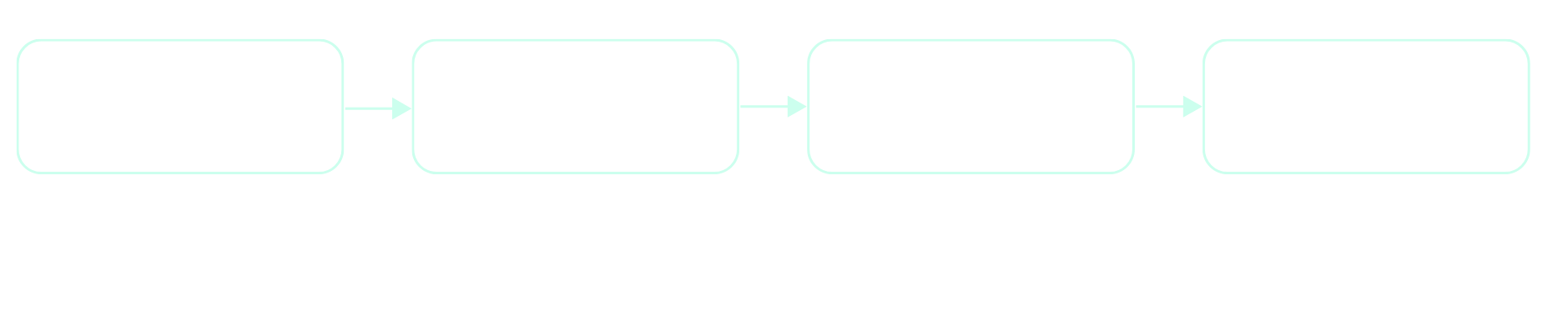
Before query optimization can occur, we need to convert the raw SQL query text to a logical query plan representation. This transformation is done in roughly three stages: SQL Parsing, SQL Validation, and SQL to Relational Algebra Conversion.
SQL Parsing: Calcite’s SQL parser transforms SQL text into an abstract syntax tree (AST). The parser is programmatically generated from a grammar specification using JavaCC. BodoSQL customizes this grammar to support Snowflake-style SQL syntax. When adding new syntax, such as DDL statements, we use Calcite’s built-in parser extension points wherever possible. However, some syntax requires changing how Calcite parses existing SQL constructs, which means modifying the core grammar directly. These changes are less ideal because they must be maintained and reconciled with changes from upstream Calcite. We’ll return to how we manage this later in the post.
SQL Validation: The SQL validator checks that a parsed query is semantically valid given the available schemas and the rules of the target SQL dialect. Because Snowflake semantics sometimes differ from Calcite’s defaults, BodoSQL extends its validator to support Snowflake-compatible semantics for functions like HASH. Where possible, we implement these customizations by extending Calcite’s SqlValidator with our own subclass; for behavior that is not exposed through Calcite’s extension points, we maintain targeted changes to the internal validator implementation. Validation also requires metadata about the tables being queried. To make that metadata available across BodoSQL’s supported data sources, we extend Calcite’s Schema interface. BodoSQL has two basic schema types: LocalSchema, for tables that exist outside a catalog, such as DataFrames and Parquet files, and CatalogSchema, which retrieves table metadata from external catalogs such as Snowflake and Iceberg.
SQL to Relational Algebra Conversion: The final step before query optimization converts the validated SQL AST into a tree of relational operators. BodoSQL extends Calcite’s SqlToRelConverter through a subclass to generate custom relational nodes for constructs such as CREATE TABLE. As in earlier stages, some behavior cannot be customized cleanly through extension points, so we also maintain targeted changes to Calcite’s internal conversion logic.
To make this pipeline concrete, let’s follow a simple query through parsing, validation and relational algebra conversion:
SELECT l_suppkey, l_extendprice * (1 - l_discount) as revenue
FROM lineitem
After the parsing stage, the SQL query is represented by an AST of SQLNode:
SqlSelect [SELECT]
├── SelectList
│   ├── SqlIdentifier: L_SUPPKEY
│   └── SqlBasicCall [AS]
│       ├── SqlBasicCall [TIMES]
│       │   ├── SqlIdentifier: L_EXTENDEDPRICE
│       │   └── SqlBasicCall [MINUS]
│       │       ├── SqlNumericLiteral: 1
│       │       └── SqlIdentifier: L_DISCOUNT
│       └── SqlIdentifier: REVENUE
└── From
    └── SqlIdentifier: LINEITEM
Next, the validator resolves the column and table references using the provided schema information:
SqlSelect
├── SelectList
│   ├── SqlIdentifier: LINEITEM.L_SUPPKEY
│   └── SqlBasicCall [AS]
│       ├── SqlBasicCall [TIMES]
│       │   ├── SqlIdentifier: LINEITEM.L_EXTENDEDPRICE
│       │   └── SqlBasicCall [MINUS]
│       │       ├── SqlNumericLiteral: 1
│       │       └── SqlIdentifier: LINEITEM.L_DISCOUNT
│       └── SqlIdentifier: REVENUE
└── From
    └── SqlBasicCall [AS]
        ├── SqlIdentifier: TPCH.LINEITEM
        └── SqlIdentifier: LINEITEM
Finally, the AST is translated into a relational tree consisting of RelNodes:
LogicalProject
├── L_SUPPKEY = $2
├── REVENUE = $5 * (1 - $6)
└── SnowflakeTableScan
    ├── Table: TPCH.LINEITEM
    └── Columns:
        $0  L_ORDERKEY
        $1  L_PARTKEY
        $2  L_SUPPKEY
        $3  L_LINENUMBER
        $4  L_QUANTITY
        $5  L_EXTENDEDPRICE
        $6  L_DISCOUNT
...At this point, BodoSQL has converted the query into a logical relational plan, but that plan describes what the query computes rather than the most efficient way to execute it. Next, it’s the optimizer's job to determine how that computation should be performed efficiently and transform the logical plan into a physical plan that BodoSQL’s execution backend can run. The optimizer pipeline consists of several stages, each of which processes a query plan before passing it to the next stage. BodoSQL configures both the stages and the order in which they run, with many stages using one of Calcite’s planners for transforming patterns within the query plan. BodoSQL uses Calcite's two primary planning strategies at different points in this pipeline:
HEP (Rule-based Planner): HEP-based stages accept a set of rules that match specific patterns within a plan and define how those patterns should be transformed into more efficient structures. These rules are applied iteratively until the plan converges or a maximum number of iterations is reached.
As an example, let’s look at how a query with multiple joins and a filter transforms during the filter pushdown pass using HEP:
SELECT
    c.c_name,
    o.o_orderkey,
    l.l_extendedprice * (1 - l.l_discount) AS revenue
FROM customer c
JOIN orders o
  ON c.c_custkey = o.o_custkey
JOIN lineitem l
  ON o.o_orderkey = l.l_orderkey
WHERE c.c_mktsegment = 'BUILDING'
Prior to this pass, the simplified plan looks like:
Filter [C_MKTSEGMENT = 'BUILDING']
└── Join
    ├── Join
    │   ├── CUSTOMER
    │   └── ORDERS
    └── LINEITEM
First, we can use a “push filter below join” rule, which pushes a filter that only depends on one side of the join into that side. Since C_MKTSEGMENT is coming from the Customers table, we can push it below the outermost join:
Join
├── Filter [C_MKTSEGMENT = 'BUILDING']
│   └── Join
│       ├── CUSTOMER
│       └── ORDERS
└── LINEITEM
After we’ve applied this rule, we can apply it again, this time on the innermost join:
Join
├── Join
│   ├── Filter [C_MKTSEGMENT = 'BUILDING']
│   │   └── CUSTOMER
│   └── ORDERS
└── LINEITEM
Finally, assuming these tables are coming from Snowflake, we can push this filter into the IO node by converting it to a SnowflakeFilter using another rule. The final plan after filter pushdown becomes:
BodoLogicalProject
└── BodoLogicalProject
    └── BodoLogicalJoin
        ├── BodoLogicalJoin
        │   ├── SnowflakeFilter
        │   │   └── SnowflakeTableScan [CUSTOMER]
        │   └── SnowflakeTableScan [ORDERS]
        └── SnowflakeTableScan [LINEITEM]
Once we can no longer apply rules or further improve the query plan, the stage ends.
Volcano (Cost-based Planner): Similar to HEP, the Volcano-based stage accepts a set of transformation rules. However, rather than simply applying rules to the current plan, Volcano uses them to explore a space of equivalent plans and a cost model to select the lowest-cost alternative.
Continuing our example from the previous section, the logical plan involves joining three tables: Lineitem, Orders, and Customers. There are multiple equivalent ways these joins could be ordered, each with a different estimated cost. For example:
           Ordering A                       Ordering B
            Cost: 200                        Cost: 300

               Join                            Join
              /    \                          /    \
           Join    LINEITEM               Join    CUSTOMER
          /    \                         /    \
     CUSTOMER  ORDERS                LINEITEM ORDERS
The planner keeps track of these alternatives and their costs and uses them to select the plan with the cheapest cost overall. In this simplified example, this corresponds to selecting the cheapest join order. The costs themselves are estimated using metadata available to the planner.
Logical to Physical Plan Conversion: BodoSQL first applies several rule-based HEP stages to simplify and optimize the logical plan before performing cost-based optimizations using Volcano. As part of producing an executable plan, BodoSQL also converts logical relational operators into physical operators that describe how the computation will be performed by its backend. Since multiple physical operators could map to the same logical operator, the logical-to-physical transformation uses Volcano and the cost-model to select the most efficient physical alternative.
Additional Optimizer Stages: After logical-to-physical conversion, BodoSQL runs additional stages to clean up and enrich the physical plan. Some use HEP, while others implement specialized BodoSQL optimizations directly.
One such specialized stage implements subplan caching, which identifies identical or similar computations that appear in multiple places in the plan and replaces them with explicit cache nodes. This indicates to the backend that these subplans can be computed once and reused during execution.
Another specialized stage implements runtime join filters (RTJFs), which use runtime values observed on the build side of a join to filter rows from the probe side, reducing unnecessary computation and I/O. During this stage, RTJF nodes are inserted after joins and pushed down towards data sources. Introducing RTJFs creates an execution dependency between the two sides of a join, meaning the plan is no longer purely relational. As a result, RTJF insertion occurs near the end of the optimizer pipeline, after transformations that rely on relational equivalence have already been performed.
These stages involve several additional considerations, including how caching interacts with RTJFs. We’ll explore these optimizations, along with other parts of BodoSQL’s optimizer pipeline, in more detail in future posts.
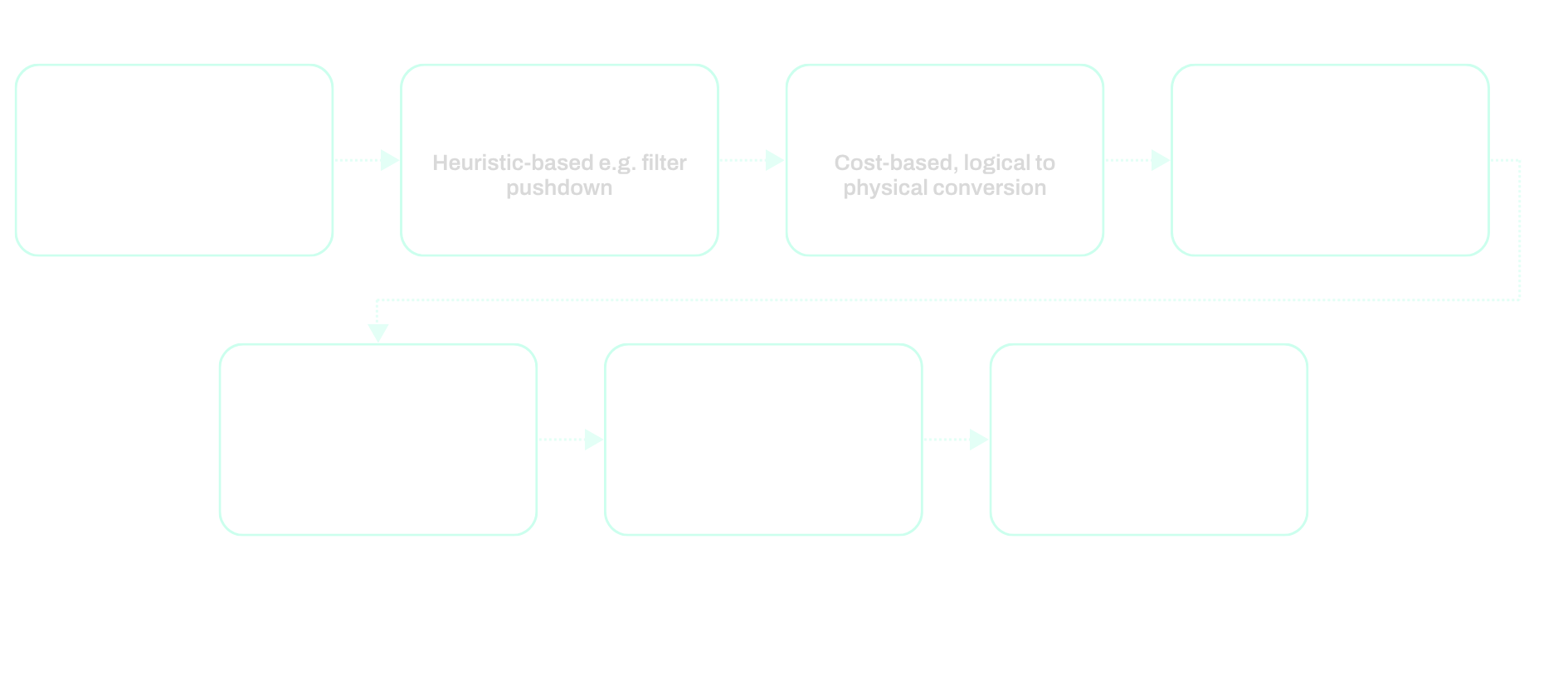
The following diagram shows where each of the stages discussed fits into the overall optimizer pipeline:
BodoSQL extends Calcite in two ways. Many customizations, such as custom optimizer rules and stages, build on Calcite’s public extension points and can live entirely within BodoSQL. Others, including changes to the core parser grammar or validator internals, require modifying Calcite itself. The latter creates an additional challenge: how do we maintain those changes while continuing to upgrade an actively developed upstream project? To maximize our productivity while mitigating issues, we use Maven Shade and the following process when modifying Calcite source files:
Bodo Change in the hopes that they can be removed if the corresponding capability becomes available upstreamWhen upgrading Calcite, we manually apply the diff to these modified files and resolve conflicts between the upstream changes and our modified sections. The process of upgrading modified files can add significant overhead, so we try to minimize these types of changes as much as possible.
BodoSQL uses Calcite as a mature foundation for its pipeline that transforms a user’s SQL query through parsing, semantic validation, and query optimization into an efficient execution plan for its high-performance backend. Many parts of Calcite are extensible enough to allow BodoSQL to define its own SQL semantics and optimization strategies while continuing to benefit from upstream improvements. Still, there remain areas where BodoSQL modifies Calcite’s internal implementation. We try to minimize these changes and the maintenance burden they introduce, and hope to reduce them further as BodoSQL continues to evolve alongside the Calcite project.
To get started using BodoSQL yourself:
And join the Community Slack to stay in the loop on product releases, new features, and other updates.